When you click on the 'Analyse' button on the CLAMP Online Analysis page (and you have set up your upload file correctly) you will generate a series of plot and data files. You will see a list of files names followed by low resolution plots of Canonical Correspondence Analysis (CCA) axes 1/2, 2/3 and 1/3.

Results Data Files

Your results are assigned a unique submission identifier that will look like something like this: '2A0F232FEE5CF9AE'.

The values of the predicted climate variables for your passive (fossil) samples are given in file 'Predicted.csv'. This can be opened in a spreadsheet such as Excel.

A copy of your uploaded scores is provided (in this case it is called 'Fossils.csv'), while the 'CCA Scores.csv' file contains all the CCA biplot scores for the calibration sites, the passive (fossil) sites and the leaf character states. The set up parameters for the analysis (i.e which calibration and output options and the name of the file that you uploaded containing the passive scores) is given in the 'params******.txt'. This text file can be opened in a word processor or text editor application and the '******' refers to the unique name of your analysis.

Results Plot Files

In the plots the positions of your unknown (passive) samples are shown in red while the positions of the calibration sites are shown as black open circles. All are identified by a number reflecting the order they appeared in the uploaded score file or calibration files. Also plotted in blue are the directions of the various climatic parameter vectors. You can use these plots to immediately see if the run has been successful (red dots will not appear if there was a problem with your uploaded score file). They will also help you to decide if any samples lie outside the physiognomic calibration space. Fossil Sample 4 (Bilyeu Creek) is a sample that does this in Figure 1, so the results for this sample will be less reliable than those for the other samples. If this occurs it may be that you made a poor choice of calibration, or that something is wrong with your scoring technique, or your fossil assemblage suffers from a strong preservational bias. Experiment to see if your fossil site is a better fit with a different physiognomic calibration. You will also see a '3D' representation of CCA axes 1-3 space. These plots are also available as higher reolution files for publication in colour or black and white in the file 'CCAGraph.pdf'.

	Figure 1. Plot of CCA axes 1 and 2 for the 'Fossils.csv' test file run with Physg3arcAZ and gridded meteorological data showing positions of passive (fossil) samples in red and the direction of the respective climate parameter vectors.

	Figure 2. Three dimensional plot of CCA axes 1, 2 and 3 for the 'Fossils.csv' test file run with Physg3arcAZ and gridded meteorological data. Note that some red (passive) sites appear to be outside physiognomic space. Results for such sites are likely to be unreliable.

 

Plots are also given of the positions of the leaf character states in relation to the climate variables. Note that these only change when the calibration files change.

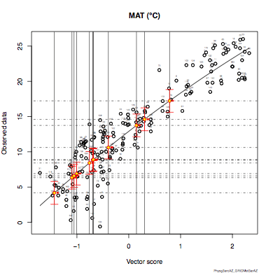
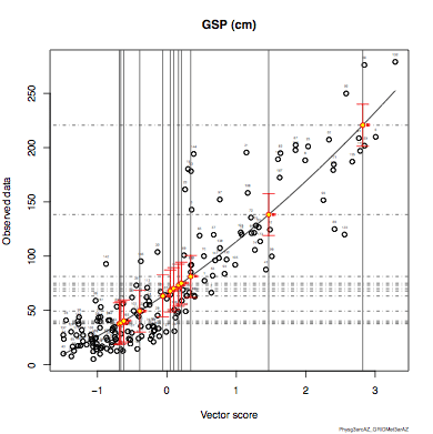
Another set of plots that are immediately available as low resolution images are the Mean Annual Temperature (MAT) and Growing Season Precipitation (GSP) regression models. The positions of the passive fossil samples along the regression line are plotted along with whisker plots in red showing the uncertainty as ± 2 sigma (standard deviations) of the residuals ablout the regression line. Again the samples are numbered for reference. These, and the regression models for all the other climate parameters, are available in higher resolution in the 'models.pdf' file.

	Figure 3. MAT regression model for the 'Fossils.csv' test file run with Physg3arcAZ and gridded meteorological data overlain with the positions along the vector score (x) axis of passive (fossil) samples in red with yellow centres. The "whiskers" indicate ± 2 sigma uncertainties. Read off the predicted climate values on the Y axis.

	Figure 4. GSP regression model for the 'Fossils.csv' test file run with Physg3arcAZ and gridded meteorological data overlain with the positions along the vector score (x) axis of passive (fossil) samples in red with yellow centres. The full span of the "whiskers" indicate ± 2 sigma uncertainties. Read off the predicted climate values on the Y axis.

 

Results Download Options

At the end of the results page there are links where all the data files and plot files in high resolution.pdf format can be downloaded.