Uncertainties in CLAMP (and other climate proxies)

For a palaeoclimate proxy to be effective it needs 1) to be internally consistant 2) have known quantified uncertainties and 3) give results that are consistant with other proxies. In regard to 3) CLAMP has been shown to yield the same or very similar results to geochemical proxies from the Cretaceous to the Neogene, and where differences exist they are systematic and consistant. For more details on this topic click here. Internal consistancy (requirement 1) in CLAMP is achieved through standardized collecting and scoring protocols coupled with the use of defined and publicly available 'open source' calibration data sets and methodologies. With respect to quantifying uncertainties (requirement 2) the CLAMP methodology automatically incorporates and quantifies a range of uncertainties. This page explores these in more detail.

CLAMP uncertainties arise from the way climate data are recorded and gridded, climate alters over time, variations in local microclimates and how plants respond to them, and how well leaf physiognomy data from a given site are collected and converted to the CLAMP scoring scheme. Uncertainties introduced through the processes of fossilization (taphonomy) and fossil collection are largely unknown and unquantifiable, but the multivariate nature of CLAMP has been shown to confer a high degree of robustness to taphonomic data loss. Unlike many proxies CLAMP has been subject to a wide range of studies examining its reliability and precision, either through experiment or by inter-proxy comparison.

Before looking at the way uncertainties are measured in CLAMP and its reliability it is worth considering the sources of uncertainties in any plant-based palaeoclimate proxy. These uncertainties can be divided into four broad categories:

1. Taphonomic - the extent to which the features being measured in the fossil assemblage are altered during the process of transport, deposition and fossilization.
2. The errors associated with the way climate, used to calibrate the proxy, is measured.
3. Uncertainties related to the natural ‘noise’ that arises from individual responses to environmental constraints.
4. Uncertainties that arise from errors in measuring the plant characteristics underpinning the proxy.

1. Taphonomic Uncertainties

In the case of CLAMP several papers have examined this, recognizing that the loss of information during the fossilization process means, by definition, that it is not measureable. However the maximum uncertainty of single or multiple character loss can be measured in extremis by seeing how much predictions are altered by loss of complete character states across all taxa, even if this means that some of the resulting estimates are highly theoretical because complete character loss would render the material unscoreable. Because CLAMP is a multivariate technique that incorporates information from across 31 character states it has proven to be remarkably robust to taphonomic losses. Empirical tests of CLAMP’s resilience to taphonomic issues were conducted by Wolfe (1993), but a statistical approach has been used by Spicer et al. (2005) and Spicer et al. (2011). Leaf Margin Analysis(LMA) is also prone to taphonomic uncertainties but is potentially more susceptible than CLAMP because of its univariate nature.

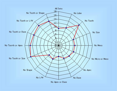This 'spidergram' shows the effect of character loss on the MAT estimate using the Physg3br data set. The scale in °C is shown on the vertical line running from the centre of the plot to the '12 o'clock' position. The complete dataset yields an MAT of 9°C. The experiment was carried out on the modern Bolshoi Canyon sample and more details can be found in Spicer et al. (2005).

 

2. Climate Measurements

Climate data are collected at standardized meteorological stations, always in clearings and, more often than not, in agriculturally modified landscapes and urban centres. The data collected this way do not record the conditions that leaves experience in, or beneath, a forest canopy. Climate, being a description of average weather, is usually framed in terms of 30-year averages or ‘normals’. Measurements are taken, sometimes hourly, across thousands of stations worldwide and inevitably the instruments used often differ, are calibrated differently, data are collected over different periods of time and often data are missing due to, for example, instrument failure or political upheaval.

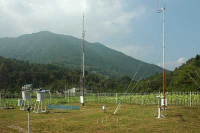Meterological stations are invariably sited in clearings or open ground and more often than not in agriculturally modified or urban landscapes. The records they make do not reflect conditions within tree crowns, forest canopies, or in the sub-canopy environment.

 

In the CLAMP MET3ar and MET3br data sets Wolfe and others tried to collect climate data close to their vegetation sites. To do this, continuous 30-year data sets were not always available and between stations different 30-year periods often had to be used.  Also, climate stations were at different distances from the vegetation sites and, although every effort was made to find climate stations at the same altitude as the vegetation site, this was not always possible. Inevitably this introduces a certain amount of variation into the data unconnected with that due to the actual climate.

To try to standardize CLAMP climate data Spicer et al.  (2009) introduced the GRIDMET3ar/br data sets. These are based on the New et al. (1999) global gridded data sets interpolated from, in the case of MAT, over 12000 meteorological stations distributed worldwide that yielded records for the 1961-1990 inclusive 30-year period. Climate stations were not uniformly distributed and so regional ‘tiling’ was used in an attempt to standardize the data. By taking data from so many stations for the same 30-year period some of the ‘noise’ in the MET3ar/br files is removed but other uncertainties are introduced. For example instrumentation and the quality of data differences are larger on a global scale than over the more restricted regional scales of the MET3ar/br datasets.

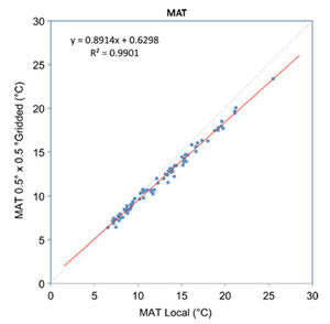
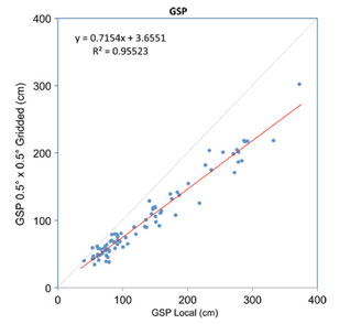
Quantifying the uncertainties in gridded data is too complex to review here but a good account is given in New et al. (1999). The largest uncertainties are associated with precipitation measurements, in part because of small-scale variations that are not captured by the spatial distribution of the meteorological stations (including biases towards easily accessible lowland sites). Moreover to correct for altitude at specific sites further spatial interpolations and altitude corrections are made (Spicer et al., 2009) that introduce additional uncertainties. These are difficult to quantify because appropriate station data are missing. Comparisons between the ungridded and gridded data are given in Yang et al. (2011) and while MAT shows a good agreement understandably precipitation measures do not. Because gridded data, with their associated uncertainties, are used in climate modelling experiments there is a strong case for using these data over the ungridded despite the larger uncertainties involved.

Graphs showing the differences in Ungridded and Gridded climate data for MAT and GSP using the MET3br (local) and GRIDMet 3br data sets. The grey line shows the ideal relationship. The Gridded GSP data are distinctly drier at higher GSP values than the Ungridded data. See Yang et al. (2011) for more details.

Within a given region climate varies both with altitude and aspect. Climate stations are often sited on flat open land and a lot of this variation is not captured and thus not reflected in gridded data. In the GRIDMET data sets some adjustment for altitude is made, but at the moment none is made for aspect. This is an area where, potentially, precision could be improved.

Leaf physiognomic adaptation to climate is made through evolutionary selection coupled with phenotypic plasticity. Aditionally species, and their foliar physiognomic spectra, are able to migrate over time and so, to some extent, track changing climates. Thus the features we score at any given site are the response to climate not in any particular year but over centuries. During that time there will be variations from year to year as well as longer term trends. We do not have instrumental records spanning evolutionary timescales, but an idea of the variation we are talking about here can be gauged from the climate trends observed over the last 130 years or more.

The changing global mean surface temperature, inter-annual variability and uncertainties since 1880. The actual variation at any vegetation site can easily be greater than the global average. (GISS/NASA)

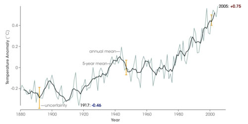
Thus the features displayed in leaf form can only approximate to the observed climate. It is also worth remembering that these variations apply equally to all climate proxies, including those based on isotopes, because they are all calibrated using observed modern climate. Inter-annual variation is likely to be less in the ocean, but ocean temperature variations are less well documented than air temperatures over land.

3. Environmental and Ecosystem 'Noise'

Spatial heterogeneity is a functional component in ecosystems and not just noise (Legendre, 1993). In plants this applies at all scales from biomes to variations in leaf form within a single tree crown and even to differences in tissue architecture, vascularization, fluid flow and diffusion pathways within leaves. Such heterogeneity is part of the spectrum of adaptation strategies that optimize fitness. In foliar physiognomic proxies this will appear, inevitably, as variations in character scores, particularly as evolution in angiosperms has resulted in selection for genomes that deliver high levels of leaf phenotypic plasticity.

In CLAMP scoring attempts to capture the full range of morphologies displayed within a species at a given site and embraces the heterogeneity that is part of ecosystem function, even though this means that correlations are not as precise as one would wish for. Such variability is, after all, likely to be present in fossil leaf assemblages.

Because often the parent plant of a fossil leaf is unknown Wolfe (1993) chose to sample all woody taxa (herbs seldom shed their leaves and thus herb leaves are only rarely found as fossils) spanning all growth forms (trees, shrubs, vines etc.).  Exclusion of any of these growth forms gives rise to error (Burnham et al., 2001). Within this spectrum of growth habit leaves from exposed sunny environments and shady sub-canopy settings are included, again because a leaf's origin with the crown/canopy cannot be routinely determined from a fossil. This sampling strategy does of course mean that CLAMP includes leaves from a wide range of microclimates experienced within the crown and canopy space. Although these microclimates track the external (free air) environment measured by meteorological stations (Fritts, 1961) they tend to be cooler and more moist than the free air due to evapotranspiration. Most of the leaves sampled in CLAMP, whether living or fossil, are derived from the cooler more humid canopy and sub-canopy environments, but include both north and south facing slopes (Spicer and Wolfe, 1987). Because CLAMP calibrations include ‘outgroup’ samples from open dry vegetation (in order to better position some moisture-related vectors) it does mean that some closed canopy samples with high soil moisture and under dry air masses will appear, at least seasonally (depending on the climate), significantly cooler than ‘observed’ meteorological data. For an exploration of this phenomenon see Spicer et al. (2011).

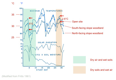Diagram from Fritts (1961) showing the reduction of sub-canopy air temperatures compared to an open site in temperate woodlands on slopes of different aspect. Conditions in the sub-canopy space track the free air temperature changes (those measured at meteorological stations) but can be up to 5 °C cooler when the free air mass is dry but the soil is wet.

A similar depression of temperature estimates and spatial heterogeneity in leaf architecture was noted by Burnham et al. (2001) when examining LMA based MAT estimates derived from river or lakeside vegetation. Again the datasets used for deriving LMA regressions are not confined to wetland vegetation and so we expect to see a similar underestimation of temperature. However, unlike CLAMP, which delivers average temperatures of the warmest month (WMMT) and coldest month (CMMT) as well as wet and dry season precipitation estimates, it is more difficult with LMA to detect when this effect comes into play and determine its magnitude.

A common source of ecosystem 'noise' that does not apply to fossils is human disturbance. This is now ubiquitous and there is a not a single vegetation type in the world that has not been directly or indirectly affected by human activity. Ideally CLAMP samples should be collected from natural or naturalised vegetation but this is not always possible. As the CLAMP database grows we can afford to be more selective and will increasingly focus on minimally disturbed vegetation.

4. Sampling and scoring ‘errors’

To maximize precision in the face of natural heterogeneity CLAMP uses several collection and scoring strategies. Collection for calibration is over a limited area. This is in order to minimize the variation in free-air climate at a sampling site. Typically this would be within 0.5 km of a central point and at the same altitude. Gregory-Wodzicki (2000) pointed out the wisdom of adopting this strategy in contrast to less constrained data derived from floral manuals that relate to taxa distributed over large, often undefined areas (e.g. Wilf et al., 1998; 1999). By restricting CLAMP sampling to small areas the climate be better defined and the range of variation in leaf characterslimited. This in turn contributes to greater precision (Wolfe and Uemura, 1999).  Taphonomic work has repeatedly shown (Burnham et al., 2001; Ferguson, 1985; Spicer, 1981; Spicer, 1989) that leaf assemblages tend to reflect local, rather than regional, vegetation and thus CLAMP sampling is designed to be analogous to the natural sampling that results in a fossil assemblage.

Nevertheless the scoring process relies on collecting the full range of leaf morphologies displayed within a species at a site and some morphologies may be overlooked. Once collected the leaf sample may be miss-scored, but experiments with novice scorers, even those speaking different languages, have shown that, following improvements in scoring instructions, this is now less of a problem than perhaps it once was (Spicer and Yang, 2010). Undoubtedly having numerous taxa scored for numerous character states minimizes the effect of miss-scoring for a given character or species. However, no amount of inbuilt robustness can overcome problems that are introduced if the CLAMP sampling or scoring protocols are not adhered to. Attempts to change the scoring regime, particularly without recalibrating CLAMP, only degrades the outcome (see Peppe et al., 2010 and compare with Spicer and Yang, 2010).

Some have argued for continuous, rather than categorical, scores particularly for such characters as leaf size. Attractive as this is in terms of limiting scoring uncertainty it unfortunately captures all the natural variation present, much of which may be ‘noise’ in the sense that small differences in large leaves are likely to have less significance than small differences in small leaves. Logarithmic transform can overcome this but so does categorical scoring. This has been clearly demonstrated in palaeoecological studies (Spicer and Hill, 1979). Computer-based automated scoring is undoubtedly attractive, but it is not yet available in a useful form.

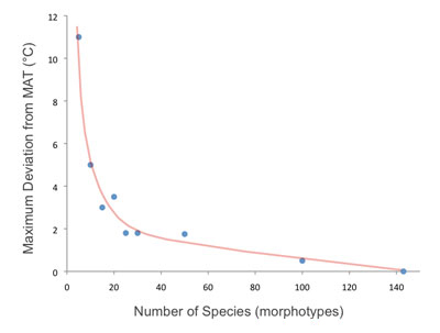
LMA and CLAMP both rely on measurements of populations of species (morphotypes) in a given area. Empirical studies have shown that for CLAMP not less than 20 species should be scored for each site (Povey et al., 1994). For LMA Steart et al. (2010) suggest no less than 15 taxa should be used.

Uncertainty reduces markedly when more than 20 species are used for each CLAMP sample. Here random subsets of different numbers of species were selected from 143 fossil species recorded at the Republic site in Washington, USA. The maximum deviation from the value derived from all 143 species reduces to zero when all species were used. (Modified from Povey et al (1994)

Measuring CLAMP uncertainties

The position of any modern day sample in a CLAMP analysis used for calibration is dependent upon biological heterogeneity in response to local environmental factors and the quality of the sampling/scoring (factors 3 and 4 above). All but 5 of the sites in the Physg3arc AZ data set have 20 or more taxa, and the minimum is 17. All leaf character states are present in all samples. This minimizes positional imprecision but nevertheless, strictly speaking, each site should actually be represented not by a point but a hyper-dimensional sphere, the diameter of which is proportional to the imprecision. Because aspects of ecological heterogeneity and failure to capture all aspects of morphological variation in scoring cannot be quantified, defining the position of each site by anything other than a point is impractical. What can be done, however, is to accept that such uncertainties exist and contribute to the scatter of the residuals about the 2nd order polynomial regression models used to calibrate CLAMP.

Uncertainties in climate measurements (see New et al. 1999 for a detailed account of these) lead to the positions of the climate vectors being only approximate. Uncertainties depend on site locations and the climate variable, but typically in that data set mean temperature errors could be as high as 1.3 °C. Such errors in the basic meterological data suggest that it is unrealistic to expect any proxy for temperature to be more precise than plus or minus 2-3 °C. This meteorological uncertainty is captured in the scatter of the CLAMP regression model residuals because the climate uncertainty for each site will be different, as will its positional relationship to the vector.  Note that such uncertainties apply to any climate-related proxy because the Earth’s climate is imperfectly characterised by station data that are the basis for gridded datasets.

Despite these uncertainties it is clear that the relationships between CLAMP leaf characters and climate are not due to chance. Monte Carlo methods available in CANOCO show that the various regressions are highly unlikely to be due to chance (p< 0.001 for many variables).

The statistical uncertainties encapsulating all sources other than taphonomic are estimated in CLAMP by means of the scatter seen in the regression models. This is the scatter of the residuals about a 2nd order polynomial regression line summarising the relationship between the climate vector scores (position along the climate vector) and the observed climate values for those sites. Thus within each calibration dataset each climate variable has its own specific uncertainty estimate. The scatter of the sites about the regression model line is usually expressed in terms of standard deviations, with ± 2 standard deviations encompassing 95% of the data. This measure, however, calculates uncertainty from the point of view of active samples and not passive ones as is the case with fossils, and only in respect of the vector score rather than the observed climate data.

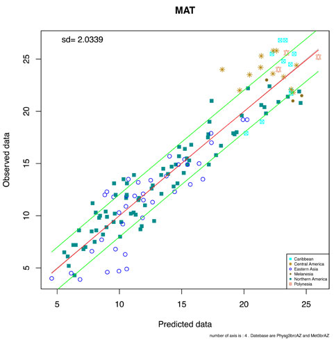
To provide a more realistic assessment of CLAMP uncertainties we removed each modern sample in turn from the data set and treated it as passive. A new regression model was then constructed based on the passive positions of each modern site in a plot of observed climate against that predicted by CLAMP. Although this increases the uncertainty values it is a fairer reflection of the uncertainties relating to fossil data. This is what should be used as the measure of precision from now on. The results of this exercise are summarized in the figure and table below.

Plot of the Physg3brcAZ samples treated as passive. Vertical axis observed MAT, horizontal axis predicted MAT. The regression line is shown in red and the green lines show 1 s.d.. Sites are coded by geographical region.

Because each modern site has a complete suite of character scores (unlike often incomplete fossils) they represent the minimum uncertainties associated with the positioning of passive samples. In practice fossil leaves are often lacking in some features due to taphonomic or collecting losses. These losses can be shown to have minimal effect even in the most extreme situations of complete loss of characters suites across all taxa (Spicer et al. 2005; 2011) in that the predicted climates arising from such character loss lie within the uncertainty range of the full data set (Spicer et al. 2005; 2011). However, this is only true if the 'completeness statistic' calculated automatically on the scoresheets remains above 0.66.

		Datasets	MAT (°C)	WMMT (°C)	CMMT (°C)	LGS (Months)	GSP (cm)	MMGSP (cm)	3-WET (cm)	3-DRY (cm)	RH (%)	SH (g/kg)	Enthalpy 0.1*(kJ/kg)
		Physg3brc + Met	2.0	2.7	3.4	1.1	48.3	5.2	20.6	13.7	11.1	1.7	0.6
		Physg3brc + GRIDMet	2.1	2.5	3.4	1.1	31.7	3.8	22.9	5.9	8.6	1.7	0.8
		Physg3arc + Met	2.8	3.1	4.0	1.3	45.0	5.0	19.4	13.2	12.7	1.8	0.6
		Physg3arc + GRIDMet	2.8	3.0	3.8	1.3	30	3.6	22.1	5.9	10.5	1.7	0.8
		PhysgAsia1+ HiResGRIDMetAsia1	2.5	3.0	4.1	1.3	49.7	5.5	23.9	10.4	7.5	1.8	0.9
		PhysgAsia2 HiResGRIDMetAsia2	2.3	2.8	3.6	1.1	60.6	6.1	35.8	9.5	8.4	1.9	0.9
		PhysgGlobal378+ HiResGRIDMetGlobal378	4.0	3.9	6.7	1.9	54.9	6.0	32.2	13	9.3	2.0	1.1
Table showing the standard deviations calculated for each climate variable and calibration data set by sequentially treating each modern vegetation sample as a passive and plotting the observed and predicted values as in the plot above. Note that these uncertainties are slightly larger than those used in the 'classic' CLAMP analyses. To download a copy of this table click here.

 

Towards the ends of the regression line, near the limits of calibrated physiognomic space, uncertainties rise, so any fossil site lying at the extremes of the calibration has larger, poorly quantified uncertainties. This is also the case for LMA. In LMA if all the leaves are entire or non-entire then the limit of the calibration has been reached and uncertainties rise to infinity.

Tests of CLAMP reliability and inter-proxy comparisons

All proxies are subject to the uncertainties in measuring modern day climate and its inherent variability, as well as those arising from the methodology used. The only way of testing proxies in deep geological time is by comparison with results from other proxies. This is an important issue because of the possibility that atmospheric carbon dioxide concentrations could, conceivably, affect CLAMP calibration, although the multivariate character of CLAMP plus experimental testing suggests that this is unlilkely (Gregory, 1996; Herman and Spicer, 1997). So far CLAMP has yielded similar results to oxygen isotope proxies both for temperature (Kennedy et al., 2002; Spicer and Herman, 2010) and (via enthalpy) altitude (Spicer et al., 2003), although more comparisons are needed. Ufnar et al. (2004) used MAT values derived from LMA, and subsequently supported by CLAMP, to derive precipitation estimates from sideritic carbonates from the Late Cretaceous of Alaska. These precipitation estimates were in accordance with a variety of qualitative proxies as well as CLAMP. CLAMP also has been tested extensively against other plant-based proxies (e.g. Yang et al., 2007; Uhl et al., 2007) and generally found to give comparable results, albeit often temperatures are slightly cooler due to the way CLAMP is calibrated and evapotranspirational cooling in closed canopy environments.

Page Top